Time Series Notes Pt. 1: Dependence, Stationarity, and Dynamic Time Warping

What a time series is

A time series is a sequence of observations indexed by time,

$$ x_1, x_2, \dots, x_T . $$

Prices, temperatures, audio, and video all take this form. In a video, each frame is one observation $x_t$, and $x_t$ is a vector. Electronic health records have the same structure, with the added difficulty that observations arrive at irregular times.

The temporal ordering of the observations is part of the information in a time series. Nearby observations are often statistically related, and this relation is called dependence. The process that generates the observations can also drift as time passes. A pattern learned from one part of the series may then fail on another part. Stationarity is the property that rules this drift out.

This post is organized around two questions. The first asks how a single series relates to itself across time. Dependence and stationarity provide the basic language for this question. The second asks how two different series should be compared. Distances and alignment methods address this problem. Both questions rely on comparisons across time.

Temporal Dependence and Stationarity

Dependence means that observations at different times are statistically related. Covariance is the basic way to describe this relation. It measures whether two quantities tend to move together. In a time series, the relevant comparison is between the process at one time and the same process at another time. This leads to the autocovariance,

$$ \gamma(h) = \mathrm{Cov}(x_t, x_{t+h}), $$

which measures dependence across a lag $h$. A positive value means that observations $h$ steps apart tend to move in the same direction. A negative value means that they tend to move in opposite directions. A value close to zero means that there is little linear dependence at that lag.

Stationarity says when this dependence can be summarized consistently. A series is called stationary when its mean does not drift over time and its autocovariance depends only on the lag $h$, not on the specific time $t$. In that case, the relationship between today and tomorrow is statistically the same as the relationship between any other pair of observations one step apart. Patterns can be estimated from one part of the series to generalize to another.

The simplest predictive model is autoregression. It writes the present as a weighted sum of the recent past plus noise,

$$ x_t = \sum_{i=1}^{p} \varphi_i \, x_{t-i} + \varepsilon_t . $$

Forecasting, in general, estimates the conditional expectation $\mathbb{E}[x_{t+1} \mid x_1, \dots, x_t]$. Modern sequence models change the estimator. The order-one autoregressive model gives a simple picture of dependence:

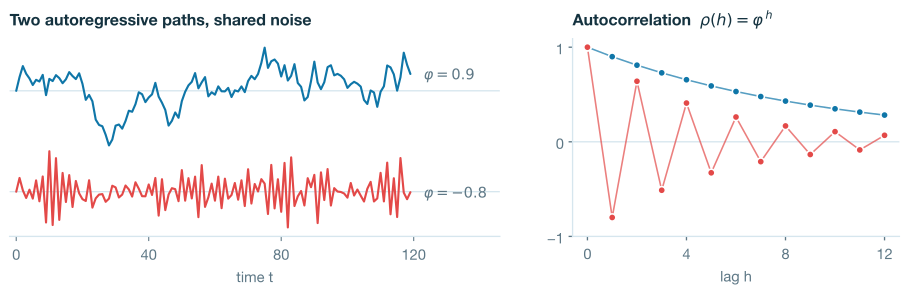
$$ x_t = \varphi x_{t-1} + \varepsilon_t . $$

Here, $\varepsilon_t$ is the new noise term at time $t$. The coefficient $\varphi$ controls how much of the previous value carries into the next one. Its sign determines the direction of dependence, while its magnitude determines the strength. When $\varphi$ is positive, high values tend to be followed by high values, and low values tend to be followed by low values. When $\varphi$ is negative, the series tends to alternate around its mean. A high value is often followed by a low one, and a low value is often followed by a high one. This behavior is visualised in Figure 1.

Two autoregressive paths driven by the same noise, next to their autocorrelation functions — Figure 1. Two autoregressive paths driven by the same noise, with the coefficient 0.9 above and the coefficient minus 0.8 below. The right panel shows the exact autocorrelation of each process. The positive coefficient gives a slow geometric decay, while the negative coefficient decays with alternating sign.

The boundary case $\varphi = 1$ is different. The model becomes

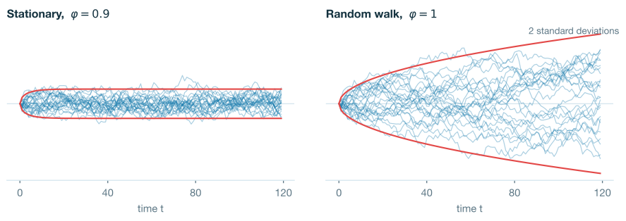
$$ x_t = x_{t-1} + \varepsilon_t . $$

Each new noise term is added to the previous level rather than gradually fading away. The series therefore wanders over time, and its variance grows as these noise terms accumulate. As a result, the process is not stationary.

Figure 2 shows the boundary case directly. Many independent paths of the stationary process settle into a band whose width stops growing, because the variance converges to $1 / (1 - \varphi^2)$. The same experiment at $\varphi = 1$ produces paths that keep spreading, because the variance at time $t$ equals $t$ itself. This distinction is a distributional one. A single realization of a random walk need not visibly display the increasing variance. The nonstationarity appears in the widening spread across repeated realizations.

Many stationary autoregressive paths inside a band of constant width, next to many random walk paths spreading without bound — Figure 2. Twenty five paths of the stationary process with coefficient 0.9 and twenty five random walk paths, driven by noise of the same scale and shown on the same vertical scale. The envelope marks two standard deviations at each time. The stationary paths settle into a band of constant width, while the random walk paths spread without bound.

Example: Bitcoin Prices

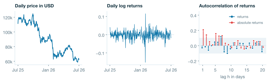
Bitcoin Prices provide a useful illustration of stationarity and dependence. Figure 3 shows one year of daily Bitcoin prices ending in July 2026. The price level drifts over time and is better viewed as a random-walk-like process than as a stationary series. Its sample mean over this period therefore does not estimate a stable long-run mean.

For this reason, financial analysis usually studies returns rather than prices. The daily log return is

$$ r_t = \log(x_t / x_{t-1}) . $$

This transformation removes the price level and describes the relative change from one day to the next. The resulting series is much closer to stationary. In Figure 3, the log returns fluctuate around zero rather than around a drifting level.

The autocorrelation of the returns is close to zero at most lags. This means that the direction of the next return is difficult to predict from recent returns alone. However, the magnitudes of the returns show a different pattern. The autocorrelation of $|r_t|$ remains positive across many lags. Large movements tend to be followed by large movements, and small movements tend to be followed by small movements. This is an important insight. A series may have little dependence in its signed changes while still having strong dependence in the size of those changes. In financial time series, this phenomenon is known as volatility clustering.

One year of daily Bitcoin prices, the daily log returns, and the autocorrelation of returns and absolute returns — Figure 3. One year of daily Bitcoin prices in United States dollars, retrieved from CoinGecko. The level drifts and is not stationary, while the log returns hover around zero. In the right panel the autocorrelation of the returns stays mostly inside the shaded band, which marks the range that uncorrelated noise would produce, while the autocorrelation of the absolute returns escapes it at many lags.

Comparing two time series

The autocovariance compared a series with a shifted copy of itself. The second question of these notes points the same idea at a new target. It asks how one series relates to another one. The Euclidean distance below performs that comparison at a fixed lag of zero. Dynamic time warping will then free the lag. Many tasks require this kind of comparison between two sequences. This includes classification, clustering, retrieval, and temporal alignment. Let

$$ X = (x_1, \dots, x_T) \qquad \text{and} \qquad Y = (y_1, \dots, y_T) $$

be two time series of the same length. A distance between them should be small when the two series represent similar behavior, and large when they represent different behavior. The simplest choice is the squared Euclidean distance,

$$ \sum_{t=1}^{T} \lVert x_t - y_t \rVert^2 . $$

This distance compares $x_t$ with $y_t$ for each time index $t$. It is appropriate when the two series are already synchronized. That assumption is often too strong. Two sequences may have the same shape but reach the same events at different times. In that case, equal indices do not necessarily represent equal progress through the underlying pattern.

Dynamic time warping (DTW) [1] relaxes the equal-index assumption. Instead of fixing the comparison between $x_t$ and $y_t$, it chooses a time-respecting correspondence between the two sequences. The correspondence must preserve order. Earlier points in one series cannot be matched to later points and then return backward in time.

Let $\pi$ denote a set of matched index pairs. The DTW distance is

$$ \mathrm{DTW}(X, Y) = \min_{\pi} \sum_{(i,j) \in \pi} \lVert x_i - y_j \rVert^2 . $$

In other words, DTW chooses the alignment that makes the paired observations as close as possible overall.

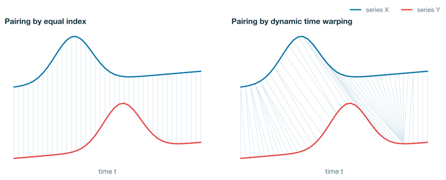
Figure 4 shows two series with a similar shape occurring at different times. The equal-index comparison pairs each observation in $X$ with the observation at the same index in $Y$. This causes the peak of $X$ to be compared with a nearly flat part of $Y$. The resulting distance is large, even though the two series differ mainly in timing. DTW gives a different comparison. It allows several nearby indices in one sequence to be matched with indices in the other sequence. This makes it possible to compare the peak of $X$ with the peak of $Y$. The two panels use the same data. Only the correspondence between indices changes.

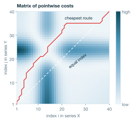
Two shifted series paired index by index, next to the same series paired by DTW — Figure 4. Two series that trace the same shape at different times, with each gray line connecting one compared pair. Equal-index pairing compares the peak of series X with a flat part of series Y. DTW pairs the peak with the peak.

The same idea can be represented as a cost matrix. For each pair of indices $(i,j)$, define the local cost $ \lVert x_i - y_j \rVert^2 . $ These costs form a matrix whose rows index one series and whose columns index the other. A valid correspondence is a path through this matrix from $(1,1)$ to $(T,T)$. The Euclidean distance corresponds to one fixed path through this matrix. It uses the diagonal path, which pairs $x_t$ with $y_t$ for every $t$. DTW instead searches over all valid paths and selects the one with the smallest total cost. This search can be computed by dynamic programming.

Figure 5 shows the cost matrix for the two series in Figure 4. The diagonal path crosses regions with large local cost, because it compares points that occur at different phases of the pattern. The DTW path bends away from the diagonal. It follows lower-cost regions of the matrix and aligns the two peaks.

The matrix of pointwise costs between two shifted series, with the equal index diagonal and the cheapest route — Figure 5. The matrix of pointwise costs between the two series of Figure 4. The equal-index pairing is the dashed diagonal. It crosses high-cost regions of the matrix. The DTW path bends away from the diagonal so that corresponding parts of the two series are compared.

Properties of DTW

The dynamic program is useful to state explicitly. Several properties of DTW follow directly from it. Let $D_{i,j}$ be the minimum alignment cost between the first $i$ points of $X$ and the first $j$ points of $Y$. Then

$$ D_{i,j} = \lVert x_i - y_j \rVert^2 + \min \left\{ D_{i-1,j},\ D_{i,j-1},\ D_{i-1,j-1} \right\}. $$

The boundary conditions are

$$ D_{0,0} = 0, \qquad D_{i,0} = \infty, \qquad D_{0,j} = \infty $$

for $i,j > 0$. The three entries inside the minimum correspond to the three possible ways to extend an alignment. The first advances in $X$ while holding the index in $Y$ fixed. The second advances in $Y$ while holding the index in $X$ fixed. The third advances in both series at the same time.

The final value $D_{T,T}$ is the DTW cost. The corresponding alignment is recovered by starting at $(T,T)$ and following the minimizing choices backward through the table. The path shown in Figure 5 is obtained in this way. The table has $T^2$ entries for two series of length $T$. Thus, computing the full cost table takes quadratic time.

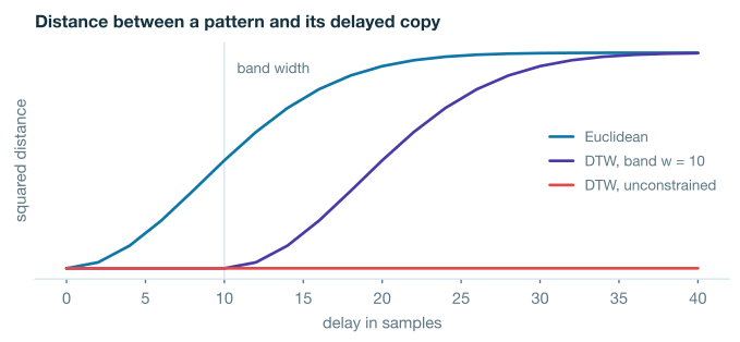
The main effect of DTW is tolerance to delays. Figure 6 compares a pattern with delayed copies of itself. The Euclidean distance increases as soon as the delay appears. It eventually stops increasing once the two patterns no longer overlap. Unconstrained dynamic time warping behaves differently. It does not require the same time indices to be compared. If the copy is delayed, the alignment can match each point of the original pattern with the corresponding point in the delayed copy. In this idealized example, the two patterns have the same values after alignment, so the dynamic time warping cost remains zero.

A constrained version gives an intermediate behavior. The banded version imposes the condition

$$ |i-j| \leq w $$

on every matched pair. This restriction keeps the alignment path within $w$ steps of the diagonal. Delays smaller than the band width can still be absorbed. Larger delays cannot. The constraint also reduces the number of table entries that must be evaluated. The running time becomes proportional to $wT$ instead of $T^2$. The band width is therefore both a computational parameter and a modeling choice. A small value of $w$ allows only limited timing differences. A large value allows stronger time distortions.

Squared distance between a pattern and its delayed copy for the Euclidean distance, banded DTW, and unconstrained DTW — Figure 6. Distance between a pattern and a delayed copy of itself as the delay grows. The Euclidean distance rises immediately. Unconstrained DTW absorbs every delay. The banded version absorbs delays up to the band width of ten samples and then rises.

This tolerance to delays also explains why DTW is not a metric. If one series is obtained from another by repeating some consecutive values, then the two series can have DTW cost zero. The repeated values can be matched to the same values in the other series without adding cost. More generally, $\mathrm{DTW}(X,Y)=0$ when the two sequences become identical after consecutive repeated values are collapsed.

This behavior is useful for alignment. A pattern and a slowed version of the same pattern should often be treated as similar. However, it is not compatible with the definition of a metric. A metric assigns positive distance to distinct objects.

DTW also violates the triangle inequality. Consider

$$ A = (0), \qquad B = (1), \qquad C = (2,2,2). $$

A direct calculation gives

$$ \mathrm{DTW}(A,B) = 1, \qquad \mathrm{DTW}(B,C) = 3, \qquad \mathrm{DTW}(A,C) = 12. $$

Therefore

$$ \mathrm{DTW}(A,C) > \mathrm{DTW}(A,B) + \mathrm{DTW}(B,C). $$

The indirect comparison through $B$ is much cheaper than the direct comparison between $A$ and $C$. Thus, DTW is symmetric and nonnegative, but it is not a metric. Methods that rely on metric structure cannot be applied with DTW. This affects some search methods, clustering algorithms, and averaging procedures. In particular, computing an exact mean of several series under DTW is NP-hard [2]. The quadratic running time is another limitation. For general DTW, this cost is difficult to improve substantially. A strongly subquadratic algorithm would contradict a standard hardness assumption in complexity theory [3].

The hard minimum in the recurrence creates a separate issue for learning. As model parameters change, the optimal alignment path can change abruptly. Gradients therefore pass only through the currently selected path and can be discontinuous when the selected path changes. This makes the hard DTW cost inconvenient as a loss function for neural networks.

Soft-DTW [4] replaces the minimum by a smooth approximation,

$$ \mathrm{softmin}_\gamma(a_1,a_2,a_3) = -\gamma \log \left( e^{-a_1/\gamma} + e^{-a_2/\gamma} + e^{-a_3/\gamma} \right), $$

where $\gamma > 0$ controls the amount of smoothing. As $\gamma$ approaches zero, the smooth approximation approaches the ordinary minimum. For positive $\gamma$, the resulting loss combines information from all valid alignment paths rather than selecting only one path. Its gradient can be computed using a related dynamic program. This gives a differentiable alignment loss that can be used to train neural networks. We will talk about this in more detail in the next blog on time-series.

Example: Bitcoin and Ethereum

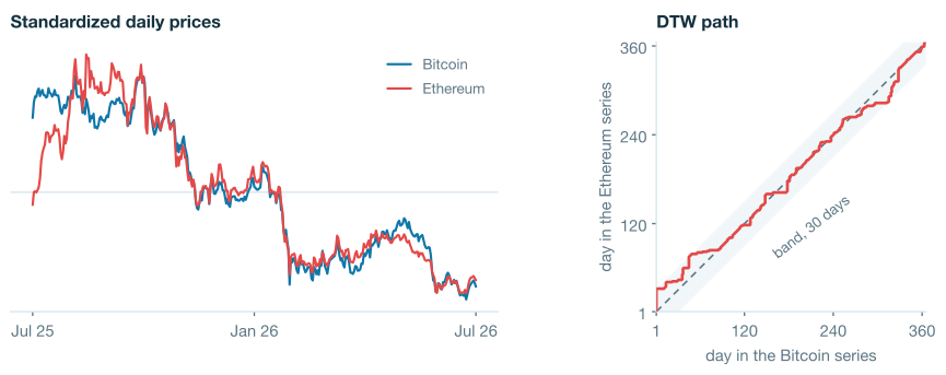
The warping distance can be put to work on the price data from Figure 3. Ethereum is the second largest cryptocurrency, and its price is widely believed to track the price of Bitcoin. Figure 7 compares one year of daily prices of the two assets. The raw levels differ by a factor of roughly forty, so each series is standardized to mean zero and unit variance before the comparison. Without this step the warping would mostly measure the gap between the price levels rather than the difference in shape. The alignment uses the banded version with $w = 30$ days.

The DTW path gives a descriptive lead-lag summary of the two markets. Points near the diagonal indicate that Bitcoin and Ethereum move in step. Points above the diagonal indicate that Bitcoin is matched to later Ethereum values, which suggests that Bitcoin leads during those periods. Over this year, the path stays close to the diagonal on average, with a mean lead of about two days. Its largest departures occur in the opening months, where the path reaches the edge of the band. The band limits the reported delay, so the true timing difference may be larger.

Standardized daily Bitcoin and Ethereum prices over one year, next to the DTW path between them inside a thirty day band — Figure 7. One year of standardized daily Bitcoin and Ethereum prices, and the DTW path between them under a band of thirty days. The path hugging the diagonal means the two markets moved nearly in step. The stretch above the diagonal in the opening months matches the Ethereum rally to Bitcoin days up to a month earlier.

The concepts from the first half of these notes can be visualized on this pair as well. Dependence between two series is measured by the cross correlation of their returns,

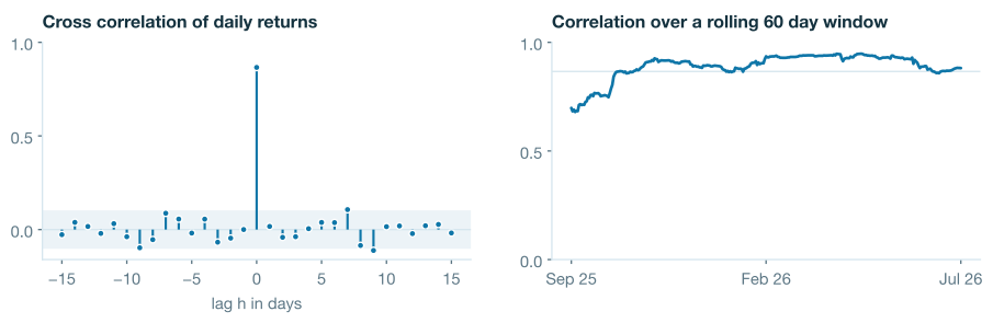
$$ \rho_{XY}(h) = \mathrm{Corr}\left(r^{X}_{t},\; r^{Y}_{t+h}\right), $$

which generalizes the autocorrelation of Figure 1 from one series to two. The left panel of Figure 8 shows this quantity for the daily returns of the two assets. The correlation at lag zero is 0.87, while every other lag stays near the noise band. The two markets move together within the same day, and neither one predicts the daily returns of the other. This does not contradict the lead found by the DTW path, because the two tools look at different objects. The path aligned slow shapes in the price levels, while the cross correlation asks whether the two series move together from one day to the next.

Stationarity of the relationship can be examined with a rolling window. The right panel of Figure 8 tracks the correlation of the two return series inside a window of sixty days. The curve stays high for most of the year, so the dependence between the two assets is roughly stable and a single number summarizes it fairly. The weakest coupling appears in the opening months, which is the same episode where the DTW path drifted furthest from the diagonal. The two views agree, and each describes the pair at a different timescale.

Cross correlation of daily Bitcoin and Ethereum returns at daily lags, next to the correlation of the two return series over a rolling sixty day window — Figure 8. Dependence between Bitcoin and Ethereum and its stability over the year. The left panel shows the cross correlation of the daily returns, with the shaded band marking the range that uncorrelated noise would produce. The correlation is 0.87 on the same day and negligible at every other lag. The right panel shows the correlation inside a rolling window of sixty days, which stays high through the year and dips only in the opening months.

Closing thoughts

These notes organized time series analysis around two related questions. The first question concerns structure within a single series. Autocorrelation addresses this question by comparing a series with a lagged version of itself. Stationarity specifies when such summaries remain stable over time. The random walk example and the Bitcoin price series show why this condition matters. When stationarity fails, averages and dependence estimates from one part of the series may not describe another part. The second question concerns comparison between two series. The Euclidean distance compares observations at equal indices. Dynamic time warping (DTW) relaxes this assumption by allowing the correspondence between indices to change. This makes it useful when two series contain similar patterns that occur at different times. These two questions are distinct, but they are connected. Autocorrelation measures dependence within one series at a fixed lag. Alignment methods compare two series by allowing the effective lag to vary over time. Both ideas treat temporal order as part of the information in the data.

References

- Sakoe and Chiba, Dynamic Programming Algorithm Optimization for Spoken Word Recognition (IEEE TASSP 1978)
- Bulteau, Froese, and Niedermeier, Tight Hardness Results for Consensus Problems on Circular Strings and Time Series (arXiv 1804.02854)
- Bringmann and Künnemann, Quadratic Conditional Lower Bounds for String Problems and Dynamic Time Warping (FOCS 2015)
- Cuturi and Blondel, Soft-DTW: a Differentiable Loss Function for Time-Series (ICML 2017)